Getting a grasp on the random walk hyperparameter
Thierry Onkelinx
2019-01-21
Source:vignettes/rwprior.Rmd
rwprior.Rmd1-D Random walks
The functions below are designed with the first order (rw1) and second order random walk (rw2) in mind. Both are one dimensional random walks. The first order random walk is defined as a random step at each point in time (\(\Delta x_i\)). All random steps are independent and identically distributed. INLA uses a zero mean Gaussian distribution with variance \(\sigma^2\).
\[\Delta x_i = x_i - x_{i - 1} \sim \mathcal{N}(0, \sigma ^ 2)\]
The second order random walk has steps defined as second order difference (the difference of differences). Here to second order differences are independent and identically distributed. INLA uses a zero mean Gaussian distribution with variance \(\sigma ^ 2\).
\[\Delta^2 x_i = \Delta x_{i + 1} - \Delta x_i \\ \Delta^2 x_i = (x_{i+1} - x_i) - (x_i - x_{i-1}) = x_{i+1} - 2 x_i + x_{i-1}\\ \Delta^2 x_i \sim \mathcal{N}(0, \sigma ^ 2)\]
Simulating random walks
Both random walks can be simulated with the simulate_rw() function. order = 1 (the default) generates first order random walks, order = 2 generates second order random walks. The hyperparameter must be specified, either as the standard error (sigma = 0.05) or as the precision (tau = 20). Another important argument is length which governs the number of time points in the time series. The default is length = 10, however it is important to set it to the length of the random walk in your model.
library(inlatools)set.seed(20181209)
# first order random walk
rw1 <- simulate_rw(sigma = 0.05, length = 20)
# second order random walk
rw2 <- simulate_rw(sigma = 0.05, length = 20, order = 2)Inspecting simulated random walks
simulate_rw() returns a data.frame with three variables: the time point x, the random walk y and the simulation replicate. The default number of simulation is 1000. You can request a different number of simulations by setting the n_sim argument in simulate_rw().
library(dplyr)
#>
#> Attaching package: 'dplyr'
#> The following objects are masked from 'package:stats':
#>
#>     filter, lag
#> The following objects are masked from 'package:base':
#>
#>     intersect, setdiff, setequal, union
glimpse(rw1)
#> Observations: 20,000
#> Variables: 3
#> $ x         <dbl> 1, 2, 3, 4, 5, 6, 7, 8, 9, 10, 11, 12, 13, 14, 15, 1...
#> $ y         <dbl> 0.00000000, 0.08202519, 0.05488452, 0.06980374, 0.04...
#> $ replicate <int> 1, 1, 1, 1, 1, 1, 1, 1, 1, 1, 1, 1, 1, 1, 1, 1, 1, 1...
Since a visual inspection is much more easy, we have defined a plot() method of the simulated random walks. This function will return a ggplot() plot, which can be fine-tuned using ggplot2 functions. The plot title displays the hyperparameter of the simulation as the standard error \(\sigma\), the variance \(\sigma^2\) and the precision \(\tau = \sigma^{-2}\). Each simulated random walk is displayed as a single line. Details on this plotting function can be found at in the helpfile of plot.sim_rw().
plot(rw1)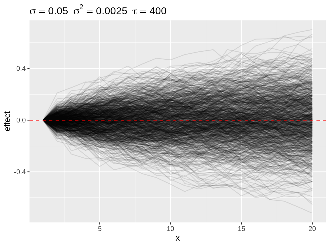
Default plot of simulated random walks applied on a first order random walk
plot(rw2)
Default plot of simulated random walks applied on the second order random walk
Summarising and subsetting
Plotting all simulations only yields a general idea on the likelihood of different effect sizes. However, plotting every simulation can be time consuming. Therefore we created a select_subset() function which calculates the quantiles over all simulations at each point in time. The user can specify the required probabilities through the quantiles argument. These default to 2.5%, 10%, 25%, 50% 75%, 90% and 97.5%. The resulting object is again a data.frame with the same structure as the simulations, which can be visuallised with the plot() function. The quantiles are useful to visalise the enveloppe of all potential random walks with that specific hyperparameter.
rw1_q <- select_quantile(rw1, quantiles = c(0.05, 0.95))glimpse(rw1_q)
#> Observations: 40
#> Variables: 3
#> $ x <dbl> 1, 1, 2, 2, 3, 3, 4, 4, 5, 5, 6, 6, 7, 7, 8, 8, 9, 9...
#> $ y <dbl> 0.00000000, 0.00000000, -0.08324475, 0.08387901, -0....
#> $ replicate <fct> 5%, 95%, 5%, 95%, 5%, 95%, 5%, 95%, 5%, 95%, 5%, 95%...
plot(rw1_q)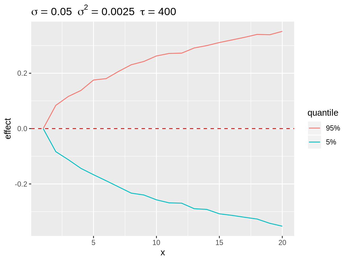
Quantiles over all simulation at each point in time displaying the enveloppe around the simulations.
select_divergence() is another option to visualise how strong the effect of the random walk can be. It selects the n (default n = 10) simulation which the strongest deviation from the baseline. The result is somewhat comparable with select_quantile() with extreme probabilities. The main difference is that select_divergence() returns a actual simulated time series.
rw1_d <- select_divergence(rw1)plot(rw1_d)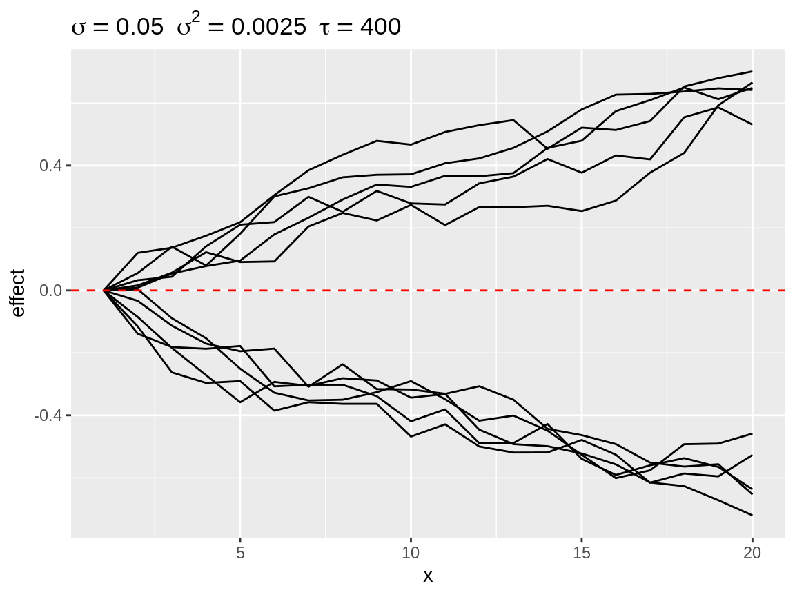
Most diverging random walks for a second order random walk process.
select_change() counts the number of changes in direction per time series. A change in direction occurs the one first order differences change sign when going from one point in time to the next point in time. The function return a selection (default n = 10) time series with the most changes in direction. These are often the most wiggly time series.
rw1_c <- select_change(rw1)plot(rw1_c)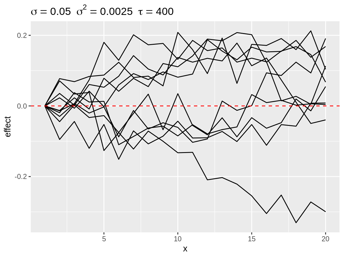
First order random walks with lots of changes in directions.
Finally, there is select_poly(). This function is useful when we assume that the random walk in the model will more or less match a pattern which can be described by a polynomial function. select_poly() fit will orthonogal polynomials see (poly()). The coefficients of the fitted polynomials compared with the user defined target coefficients. The target coefficients are rescaled to that there norm equals 1. The fitted coefficients are rescaled by a common factor so that the largest norm equals 1.
rw1_s1 <- select_poly(rw1, coefs = c(1))
rw1_s2 <- select_poly(rw1, coefs = c(0, -1))
rw1_s3 <- select_poly(rw1, coefs = c(0, 1)) plot(rw1_s1)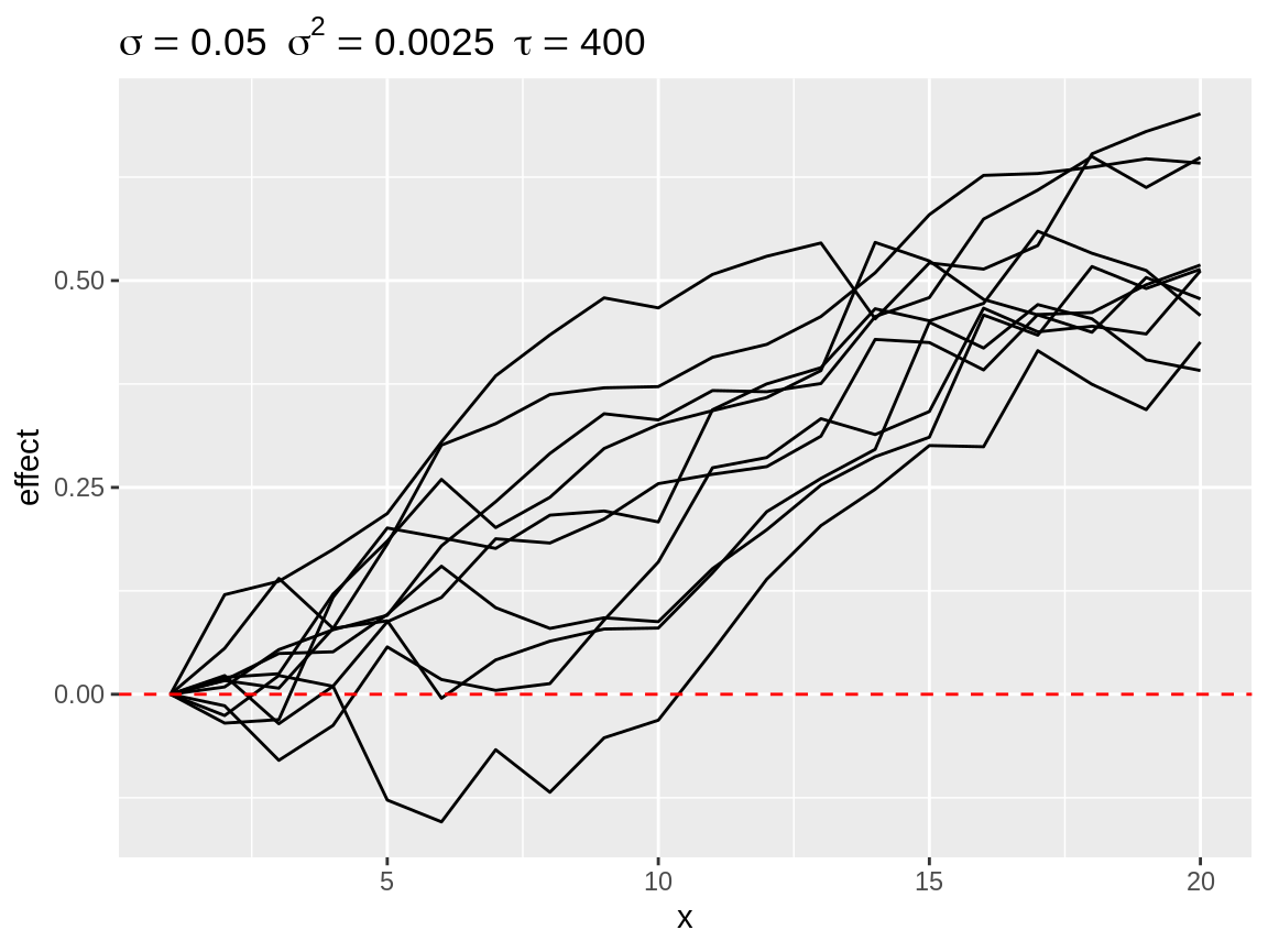
Simulated random walks best matching coefs = 1
plot(rw1_s2)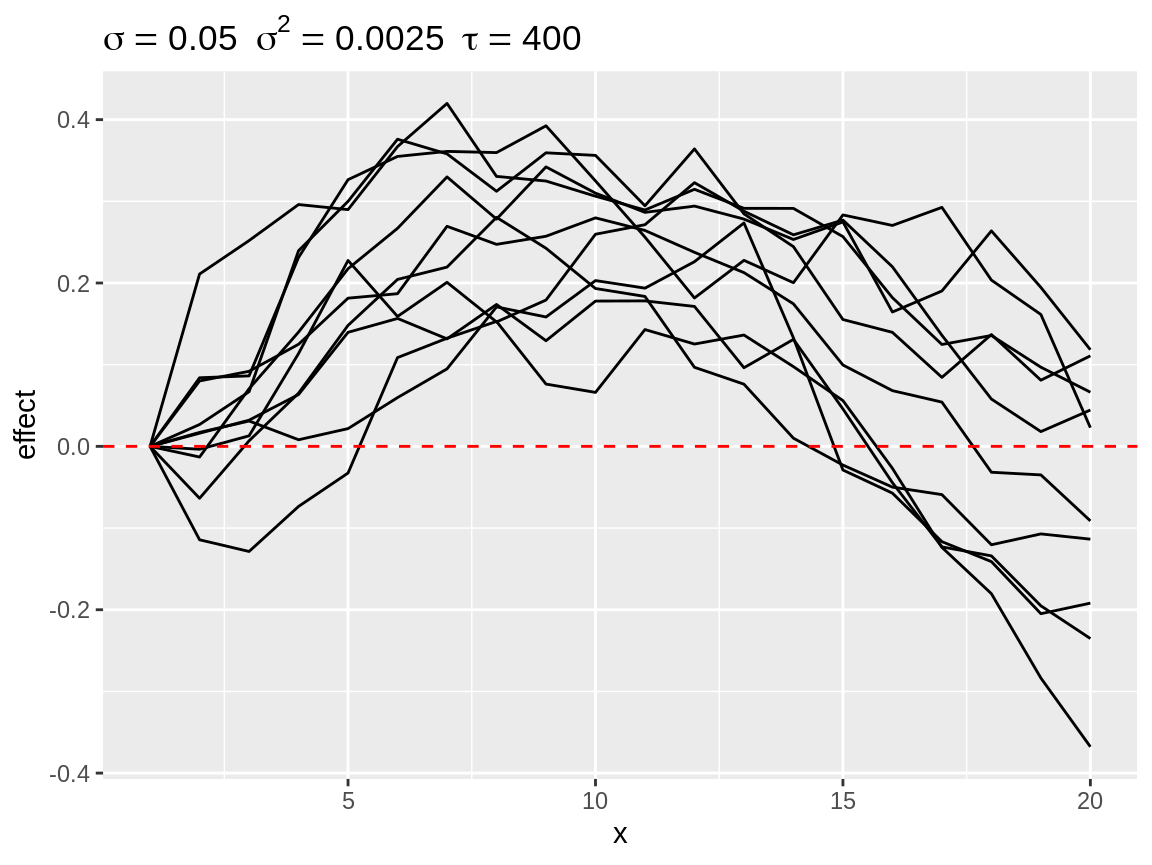
Simulated random walks best matching coefs = c(0, -1)
plot(rw1_s3)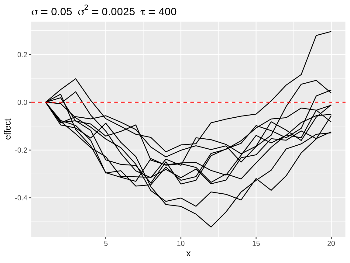
Simulated random walks best matching coefs = c(0, 1)
An attentive reader might have noticed that the different subsetting functions result in the selection of random walk with a different range although they all share the same hyperparameter. Therefore we recommend to ponder on the kind on random walk pattern you can expect from the data and use that information to choose between the subsetting functions. Is a quasi linear pattern plausible? Then select_diverging() is probably the most useful function. Do you expect a seasonal pattern with a single peak in the middle? Then select_poly() with coefs = c(0, -1) is the way to go. Frequent oscilations around a baseline? Check out select_change(). You don’t have a clue? Do some more research on the topic you are modelling, talk with domain experts and do some exploratory data analysis. Then come back to this vignette.
Baseline
Each plot has a horizontal red dashed line: the baseline. Each simulation is displayed as the random walk + the baseline. The default baseline is 0. The user can specify one or more custom baselines through the baseline argument of the plot() function. Each baseline will have its own subplot to avoid overplotting.
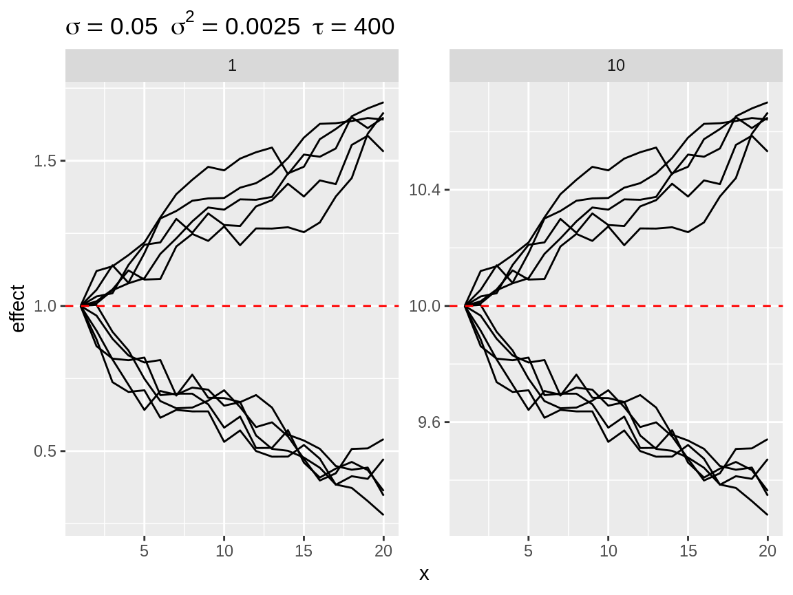
Plot divergent random walks against two baselines.
Transformations
Random effect are often applied in model that use a link function between the linear predictor and the parameter of the distribution. Think of the log-link with a Poisson or negative binomial distribution and the logit-link with a binomial distribution. Setting the link argument while plot will apply the back-transformation. Setting the link will also change the default baseline: baseline = 1 for link = "log" and baseline = c(0.05, 0.1, 0.25, 0.5) for link = "logit". We use several baseline values for link = "logit", because the effect of the random walk, in terms of absolute difference in proportion, will depend on the baseline value. Note that the baseline value is expressed on the scale of the observations.
plot(rw1_d, link = "log")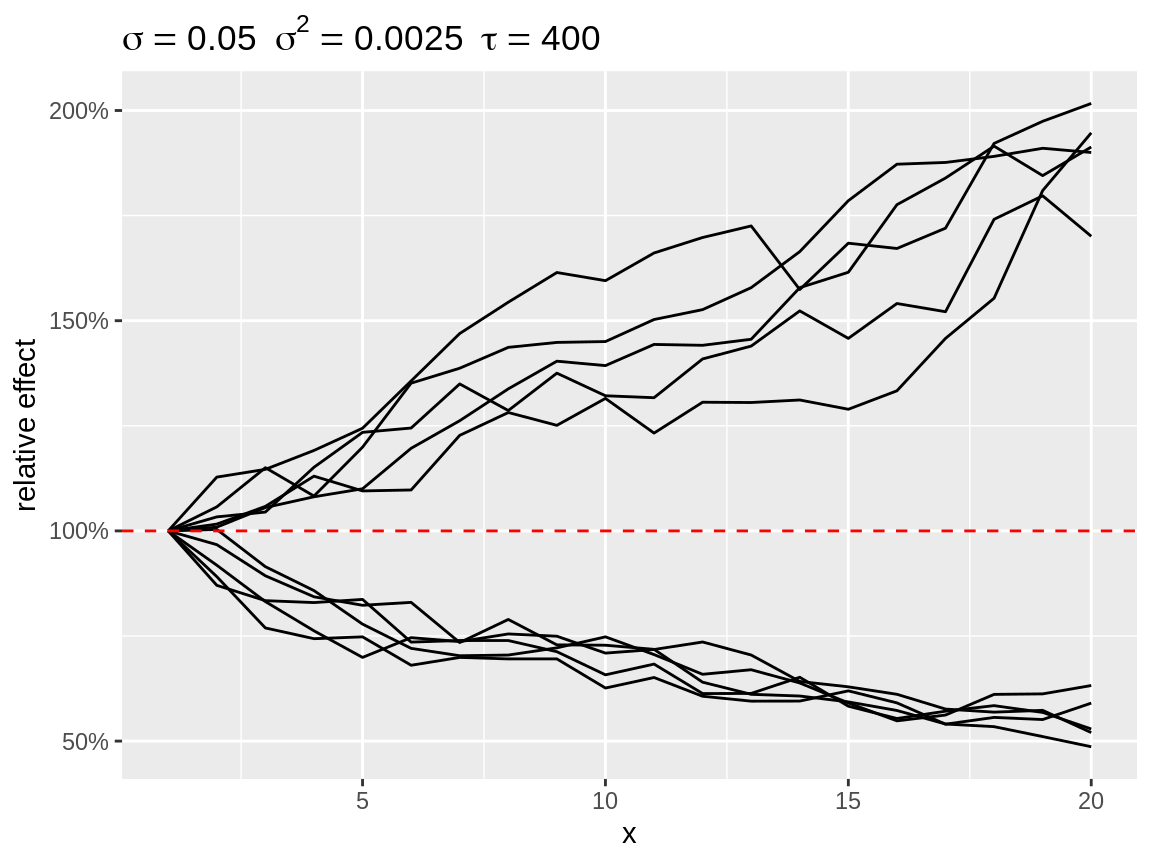
Divergent random walks with a log-link back-transformation
plot(rw1_d, link = "logit")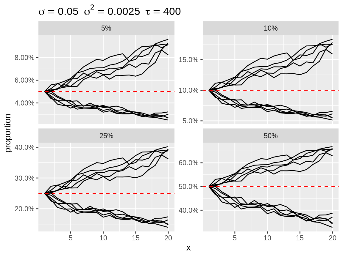
Divergent random walks with a logit-link back-transformation
Centering
By default the start of each random walk is centered on the baseline. This makes it easy to see how strong the cumulative change can be over the length of the random walk. Other options are “mean”, “bottom” and “top.” “mean” implies centering the random walk to a zero-mean effect before adding the baseline. This zero-mean centering is what INLA applies to the random walk during this model fitting. “bottom” centering fixes the lowest value of the random walk to the baseline. This make is easy to inspect the total range of the random walk. “top” does the same thing while fixing the highest value to of the random walk to the baseline.
plot(rw1_s2, center = "mean")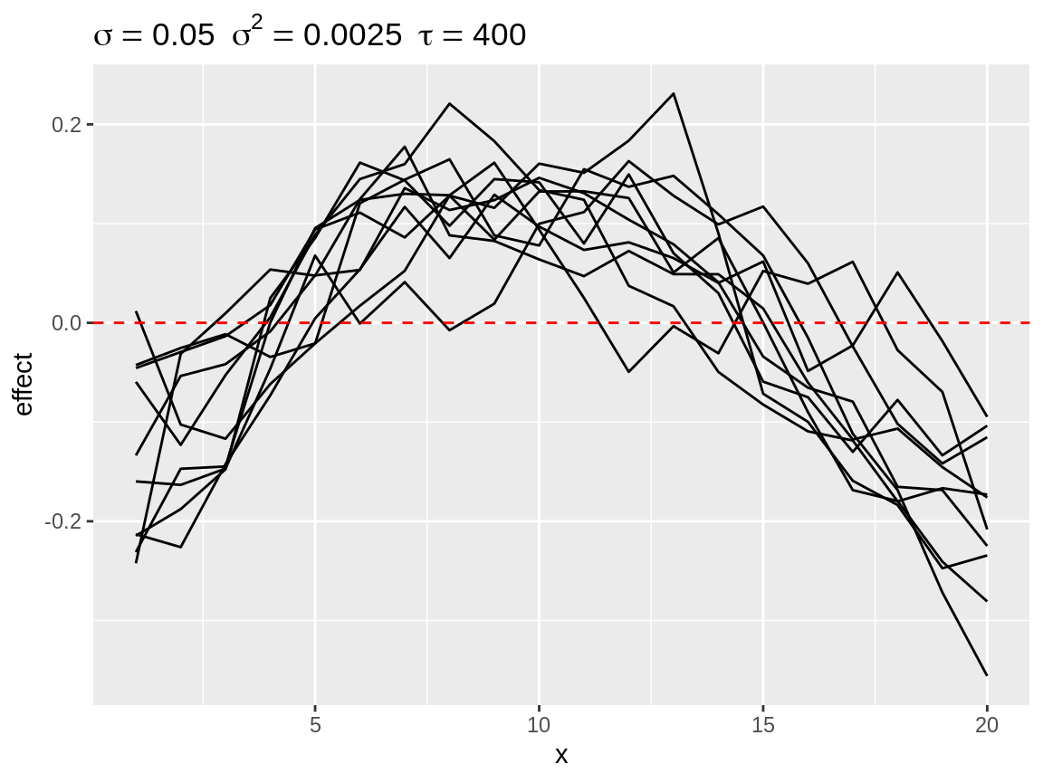
Second degree polynomial random walks with mean centering
plot(rw1_c, center = "bottom", link = "log")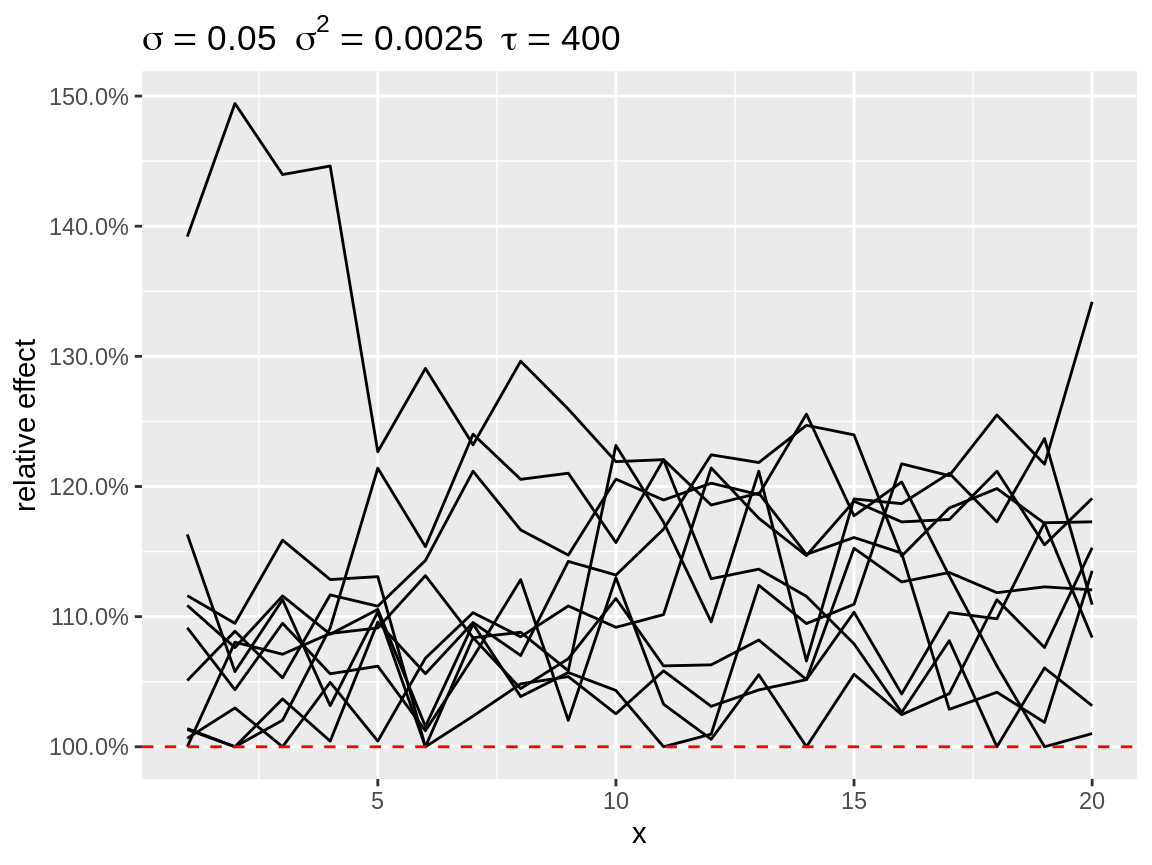
First order random walks with lots of changes in directions after centering to the bottom.
plot(rw1_c, center = "top", link = "logit")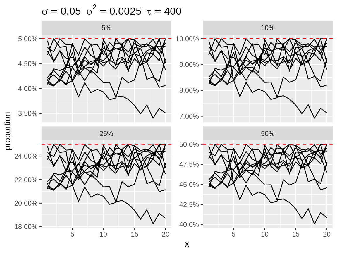
First order random walks with lots of changes in directions after centering to the top.